6. Key concepts

The OpenWFS framework is built around the concept of devices. Devices can be detectors, which capture, process, or synthesize data, or actuators, which change the state of the system. The framework provides a common interface for working with detectors and actuators, and for synchronizing their operations.

In addition, OpenWFS maintains metadata and units for all data arrays and properties where relevant. This approach reduces the chance of errors caused by passing a quantity in incorrect units, and to simplify the computation of coordinates (see Section 6.5).

6.1. Detectors

Detectors in OpenWFS are objects that capture, generate, or process data. A Detector object may correspond to a physical device such as a camera, or it may be a software component that generates synthetic data (see Section 8). Currently, the following detectors are supported:

devices.Camera	Supports all GenICam/GenTL cameras.
devices.ScanningMicroscope	Laser scanning microscope using galvo mirrors and National Instruments data acquisition card.
simulation.SimulatedWFS	Simulated detector for testing wavefront shaping algorithms.
simulation.Microscope	Fully simulated microscope, including aberrations, diffraction limit, and translation stage.
simulation.StaticSource	Returns pre-set data, simulating a static source.
simulation.NoiseSource	Generates uniform or Gaussian noise as a source.

All detectors derive from the Detector base class. and have the following properties and methods:

class Detector(Device):

    # starting a measurement
    def read(self) -> np.ndarray
    def trigger(self, out: Optional[np.ndarray] = None) -> Future

    # metadata
    data_shape: tuple[int, ...]
    pixel_size: Optional[Quantity]
    extent: Quantity
    def coordinates(dimension: int) -> Quantity

The read() method of a detector starts a measurement and returns the captured data. It triggers the detector and blocks until the data is available. Data is always returned as numpy array [33]. Subclasses of Detector typically add properties specific to that detector (e.g. shutter time, gain, etc.). In the simplest case, setting these properties and calling read() is all that is needed to capture data. The trigger() method is used for asynchronous measurements as described below. All other properties and methods are used for metadata and units, as described in Section 6.5.

The detector object inherits some properties and methods from the base class Device. These are used by the synchronization mechanism to determine when it is safe to start a measurement, as described in Section 6.6.

6.1.1. Asynchronous measurements

read() blocks the program until the captured data is available. This behavior is not ideal when multiple detectors are used simultaneously, or when transferring or processing the data takes a long time. In these cases, it is preferable to use trigger(), which initiates the process of capturing or generating data and returns directly. The program can continue operation while the data is being captured/transferred/generated in a worker thread. While fetching and processing data is underway, any attempt to modify a property of the detector will block until the fetching and processing is complete. This way, all properties (such as the region of interest) are guaranteed to be constant between the calls to trigger() and the moment the data is actually fetched and processed in the worker thread.

The asynchronous measurement mechanism can be seen in action in the StepwiseSequential algorithm used in Listing 3.1. The execute() function of this algorithm is implemented as

def execute(self) -> WFSResult:
    phase_pattern = np.zeros((self.n_y, self.n_x), 'float32')
    measurements = np.zeros((self.n_y, self.n_x, self.phase_steps, *self.feedback.data_shape))

    for y in range(self.n_y):
        for x in range(self.n_x):
            for p in range(self.phase_steps):
                phase_pattern[y, x] = p * 2 * np.pi / self.phase_steps
                self.slm.set_phases(phase_pattern)
                self.feedback.trigger(out=measurements[y, x, p, ...])
            phase_pattern[y, x] = 0

    self.feedback.wait()
    return analyze_phase_stepping(measurements, axis=2)

This code performs a wavefront shaping algorithm similar to the one described in [2]. In this version, there is no pre-optimization. It works by cycling the phase of each of the n_x × n_y segments on the SLM between 0 and 2π, and measuring the feedback signal at each step. self.feedback holds a Detector object that is triggered, and stores the measurement in a pre-allocated measurements array when it becomes available. It is possible to find the optimized wavefront for multiple targets simultaneously by using a detector that returns an array of size feedback.data_shape, which contains a feedback value for each of the targets.

The program does not wait for the data to become available and can directly proceed with preparing the next pattern to send to the SLM (also see Section 6.6). After running the algorithm, wait() is called to wait until all measurement data is stored in the measurements array, and the utility function analyze_phase_stepping is used to extract the transmission matrix from the measurements, as well as a series of troubleshooting statistics (see Section 9).

Note that, except for this asynchronous mechanism for fetching and processing data, OpenWFS is not designed to be thread-safe, and the user is responsible for guaranteeing that devices are only accessed from a single thread at a time.

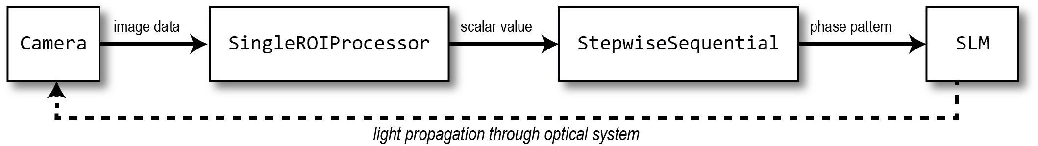
Fig. 6.1 Flowchart of the hello_wfs.py example.

6.2. Processors

A Processor is an object that takes input from one or more other detectors, and combines/processes this data. By itself, a processor is a Detector, enabling multiple processors to be chained together to combine their functionality. We already encountered an example in Section 3, where the SingleRoiProcessor was used to average the data from a camera over a region of interest. A block diagram of the data flow of this code is shown in Fig. 6.1. The OpenWFS currently includes the following processors:

processors.SingleRoi	Averages signal over a single ROI.
processors.MultipleRoi	Averages signals over multiple regions of interest (ROIs).
processors.CropProcessor	Crops data from the source to a region of interest.
processors.TransformProcessor	Performs affine transformations on the source data.
simulation.GaussianNoise	Adds Gaussian noise to the source data.
simulation.ADCProcessor	Simulates an analog-digital converter, including optional shot-noise and readout noise.

6.3. Actuators

Actuators are devices that move things in the setup. This can be literal, such as moving a translation stage, or a virtual movement, like an SLM that takes time to switch to a different phase pattern. All actuators are derived from the common Actuator base class. Actuators have no additional methods or properties other than those in the Device base class. A list of actuators currently supported by OpenWFS can be found in the table below.

devices.SLM	Controls and renders patterns on a Spatial Light Modulator (SLM) using OpenGL
simulation.SLM	Simulates a phase-only spatial light modulator, including timing and non-linear phase response.
simulation.XYStage	Simulates a translation stage, used in Microscope.

6.4. Algorithms

OpenWFS comes with a number of wavefront shaping algorithms already implemented, as listed in the table below. Although these algorithms could have been implemented as functions, we chose to implement them as objects, so that the parameters of the algorithm can be stored as attributes of the object. This simplifies keeping the parameters together in one place in the code, and also allows the algorithm parameters to be accessible in the Micro-Manager graphical user interface, see Section 10.

algorithms.FourierDualReference	A dual reference algorithm that uses plane waves from a disk in k-space for wavefront shaping [15].
algorithms.DualReference	A generic dual reference algorithm with a configurable basis set [34].
algorithms.SimpleGenetic	A simple genetic algorithm for optimiziang wavefronts [35].
algorithms.StepwiseSequential	A simplified version of the original wavefront shaping algorithm [2], with pre-optimization omitted.

All algorithms are designed to be completely hardware-agnostic, so that the exact same code can be used with any type of feedback signal on real or simulated hardware. All algorithms except the SimpleGenetic algorithm provide support for optimizing multiple targets simulaneously in a single run of the algorithm.

6.5. Units and metadata

OpenWFS consistently uses astropy.units [36] for quantities with physical dimensions, which allows for calculations to be performed with correct units, and for automatic unit conversion where necessary. Importantly, it prevents errors caused by passing a quantity in incorrect units, such as passing a wavelength in micrometers when the function expects a wavelength in nanometers. By using astropy.units, the quantities are converted automatically, so one may for example specify a time in milliseconds, minutes or days. The use of units is illustrated in the following snippet:

import astropy.units as u
c = Camera(...)
c.exposure = 10 * u.ms
c.exposure = 0.01 * u.s  # equivalent to the previous line
c.exposure = 10 # raises an error, since the unit is missing

In addition, OpenWFS allows attaching pixel-size metadata to data arrays using the functions set_pixel_size(). Pixel sizes can represent a physical length (e.g. as in the size pixels on an image sensor), or other units such as time (e.g. as the sampling period in a time series). OpenWFS fully supports anisotropic pixels, where the pixel sizes in the x and y directions are different.

The data arrays returned by the read() function of a detector have pixel_size metadata attached whenever appropriate. The pixel size can be retrieved from the array using get_pixel_size(), or obtained from the pixel_size attribute directly. As an alternative to accessing the pixel size directly, get_extent() and extent provide access to the extent of the array, which is always equal to the pixel size times the shape of the array. Finally, the convenience function coordinates() returns a vector of coordinates with appropriate units along a specified dimension of the array.

6.6. Synchronization

When running an experiment, it is essential to synchronize detectors and actuators. For example, starting an acquisition on a camera while the spatial light modulator (SLM) is still switching to a new phase pattern will result in an incorrect measurement. Similarly, moving a translation stage while the camera is still acquiring data will result in a blurred image. OpenWFS provides fully automatic synchronization between different devices, so that there is no need for manual synchronization code or sleep statements.

The Device base class implements a set of properties and methods to implement the synchronization mechanism:

class Device:
    def busy(self) -> bool
    def wait(self, up_to: Optional[Quantity[u.ms]] = None)

    duration: Quantity[u.ms]
    latency: Quantity[u.ms]
    timeout: Quantity[u.ms]

Each device can either be busy or ready, and this state can be polled by calling busy(). Detectors are busy as long as the detector hardware is measuring. Actuators are busy when they are moving, about to move, or settling after movement. OpenWFS automatically enforces two conditions:

• before starting a measurement, wait until all motion is (almost) completed

• before starting any movement, wait until all measurements are (almost) completed

Here, ‘almost’ refers to the fact that devices may have a latency. Latency is the time between sending a command to a device, and the moment the device starts responding. An important example is the SLM, which typically takes one or two frame periods to transfer the image data to the liquid crystal chip. Such devices can specify a non-zero latency attribute. When specified, the device ‘promises’ not to do anything until latency milliseconds after the start of the measurement or movement. When a latency is specified, detectors or actuators can be started slightly before the devices of the other type (actuators or detectors, respectively) have finished their operation. For example, this mechanism allows sending a new frame to the SLM before the measurements of the current frame are finished, since it is known that the SLM will not respond for latency milliseconds anyway. This way, measurements and SLM updates can be pipelined to maximize the number of measurements that can be done in a certain amount of time. To enable these pipelined measurements, the Device class also provides a duration attribute, which is the maximum time interval between the start and end of a measurement or actuator action.

This synchronization is performed automatically. If desired, it is possible to explicitly wait for the device to become ready by calling wait(). To accommodate taking into account the latency, this function takes an optional parameter up_to, which indicates that the function may return the specified time before the device hardware is ready. In user code, it is only necessary to call wait when using the out parameter to store measurements in a pre-defined location (see Section 6.1.1 above). A typical usage pattern is illustrated in the following snippet:

frames1 = np.zeros((P, *cam1.data_shape))
frames2 = np.zeros((P, *cam2.data_shape))
for p in range(P)
    # wait for all measurements to complete (up to the latency of the slm)
    # then send the new pattern to the SLM hardware
    slm.set_phases(phase * 2 * np.pi / P)

    # wait for the image on the SLM to stabilize, then trigger the measurement.
    cam1.trigger(out = frames1[n, p, ...])

    # directly trigger cam2, since we already are in the 'measuring' state.
    cam2.trigger(out = frames2[n, p, ...])

cam1.wait() # wait until camera 1 is done grabbing frames
cam2.wait() # wait until camera 2 is done grabbing frames

Finally, devices have a timeout attribute, which is the maximum time to wait for a device to become ready. This timeout is used in the state-switching mechanism, and when explicitly waiting for results using wait() or read().