7. Spatial Light Modulators

Spatial Light Modulators are the heart of any wavefront shaping experiment. Currently, OpenWFS supports the use of phase-only spatial light modulators through the following simple interface:

class PhaseSLM(ABC):
    def set_phases(self, values: ArrayLike, update: bool = True)
    def update(self)

The set_phases() method takes a scalar or a 2-D array of phase values in radians, which is wrapped to the range [0, 2π) and displayed on the SLM. This function calls update() by default to send the image to the SLM hardware. In more advanced scenarios, like texture blending (see below), it can be useful to postpone the update by passing update=False and manually cal update() later. The algorithms in OpenWFS only access SLMs through this simple interface. As a result, the details of the SLM hardware are decoupled from the wavefront shaping algorithm itself.

Currently, there are two implementations of the PhaseSLM interface. The simulation.SLM is used for simulating experiments and for testing algorithms (see Section 8). The hardware.SLM is an OpenGL-accelerated controller for using a phase-only SLM that is connected to the video output of a computer. The SLM can be created in windowed mode (useful for debugging), or full screen. It is possible to have multiple windowed SLMs on the same monitor, but only one full-screen SLM per monitor. In addition, the SLM implements some advanced features that are discussed below.

At the time of writing, SLMs that are controlled through other interfaces than the video output are not supported. However, the interface of the PhaseSLM class is designed to accommodate these devices in the future. Through this interface, support for intensity-only light modulators (e.g. Digital Mirror Devices) operating in phase-modulation mode (e.g. [37]) may also be added.

7.1. Texture mapping and blending

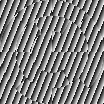
Fig. 7.1 Sample output of the SLM object, generated by the script examples/slm_disk.py. Here, two patches were used: a circular one with large segments in concentric rings, and a second one showing a superposed phase gradient.

On top of the basic functionality, the hardware.SLM object provides advanced functionality for controlling how the pixels in the phase array are mapped to the screen. This functionality uses the texture mapping capabilities of the graphics card (see, e.g. [38]) to allow for arbitrary transformations of phase maps to the screen.

Texture mapping involves two components: a texture and a geometry, which are stored together in a Patch object. The texture is a 2-D array holding phase values in radians. Values in the texture are referenced by texture coordinates ranging from 0 to 1. The geometry describes a set of triangles that is drawn to the screen, with each triangle holding a 2-D screen coordinate and a 2-D texture coordinate. The screen coordinate determines where the vertex is drawn on the screen, and the texture coordinate determines which pixel in the texture is used to color the vertex. When drawing the triangles, OpenGL automatically interpolates the texture coordinates between the vertices, and looks up the nearest value in the phase texture.

In the simplest form, a square texture is mapped to a square region on the screen. This region is comprised of two triangles, with the screen coordinates corresponding to the vertices of the square. The vertices hold texture coordinates ranging from (0,0) to (1,1). This way, the graphics hardware automatically scales the texture to fit the region, regardless of how many elements the phase map has.

A more advanced example is shown in Fig. 7.1, where the texture is mapped to a disk. The disk is drawn as a set of triangles, with the screen coordinates corresponding to points on the concentric rings that form the disk. In this example, the texture was a 1 × 18 element array with random values. The texture coordinates were defined such that the elements of this array are mapped to three concentric rings, consisting of 4, 6, and 8 segments, respectively (see Listing 7.1). Such an approach can be useful for equalizing the contribution of different segments on the SLM [9].

The example in Fig. 7.1 also demonstrates a second capability of the SLM object, namely using multiple patches simultaneously on a single SLM. The patches are drawn in the order they are present in the patches list. At the pixels where the patches overlap, the phase values for the two patches are added and wrapped to the interval [0, 2π). In the example, the first patch describes the disk, and a second square patch was drawn on top of it. This second patch holds a linear gradient, which may be used to steer the light coming from the SLM.LM, while the disk texture determines the shape of the wavefront. This blending behavior can be disabled by setting additive_blend = False, in which case each patch just overwrites the pixels drawn by previous patches.

Listing 7.1 slm_disk. Illustration of texture warping and blending functionality of the hardware.SLM object.

"""
SLM disk
=============
This script demonstrates how to create a circular geometry on an SLM
and superpose a gradient pattern on it.
"""

import cv2
import numpy as np

from openwfs.devices.slm import SLM, Patch, geometry
from openwfs.utilities import patterns

# construct a windowed-mode, square SLM window
slm_size = (400, 400)
slm = SLM(monitor_id=0, shape=slm_size)

# for the first patch, use a circular geometry, where a 1-D texture is mapped
# onto a set of concentric rings. Display a gradient pattern
shape = geometry.circular(radii=(0, 0.4, 0.7, 1.0), segments_per_ring=(4, 6, 8))
slm.patches[0].geometry = shape
phases = np.random.uniform(low=0, high=30, size=(1, 18))
slm.patches[0].set_phases(phases, update=False)

# add a second patch that corresponds to a linear gradient
gradient = patterns.tilt(slm_size, (10, 25))
slm.patches.append(Patch(slm))
slm.patches[1].set_phases(gradient)

# read back the pixels and store in a file
pixels = slm.pixels.read()
cv2.imwrite("slm_disk.png", pixels)

The combination of texture mapping and blending allows for a wide range of use cases, including:

• Aligning the size and position of a square phase map with the illuminating beam.

• Correcting phase maps for distortions in the optical system, such as barrel distortion.

• Using two parts of the same SLM independently. This feature is possible because each Patch object can independently be used as a PhaseSLM object.

• Blocking part of a wavefront by drawing a different patch on top of it, with additive_blend = False.

• Modifying an existing wavefront by adding a gradient or defocus pattern.

• Compensating for curvature in the SLM and other system aberrations by adding an offset layer with additive_blend = True to compensate for these aberrations.

All of these corrections can be done in real time using OpenGL acceleration, making the SLM object a versatile tool for wavefront shaping experiments.

A final aspect of the SLM that is demonstrated in the example is the use of the pixels attribute. This attribute holds a virtual camera that reads the gray values of the pixels currently displayed on the SLM. This virtual camera implements the Detector interface, meaning that it can be used just like an actual camera. This feature is useful, e.g., for storing or checking the images displayed on the SLM.

For debugging or demonstration purposes, it is often useful to receive feedback on the image displayed on the SLM. In Windows, this image can be see by hovering over the program icon in the task bar. Alternatively, the combination Ctrl + PrtScn can be used to grab the image on all active monitors. For demonstration purposes, the clone() function can be used to create a second SLM window (typically placed in a corner of the primary screen), which shows the same image as the original SLM. This technique is demonstrated in the wfs_demonstration_experimental.py code available in the online example gallery [39].

7.2. Lookup table

Even though the SLM hardware itself often includes a hardware lookup table, there usually is no standard way to set it from Python, making switching between lookup tables cumbersome. The OpenGL-accelerated lookup table in the SLM object provides a solution to this problem, which is especially useful when working with tunable lasers, for which the lookup table needs to be adjusted often. The SLM object has a lookup_table property, which holds a table that is used to convert phase values from radians to gray values on the screen. By default, this table is set to range(2 ** bit_depth), meaning that if an 8-bit video mode is selected, a phase of 0 produces a gray value of 0, and a phase of 255/256·2π produces a gray value of 255. A phase of 2π again produces a gray value of 0.

7.3. Synchronization

When working with an SLM that is connected to a video output, it is essential to synchronize with the vertical retrace of the graphics card. ‘Vertical retrace’ is the historical name for the start of a new frame. The software should update the image on the screen only during this vertical retrace. If the image is changed between vertical retraces, tearing will occur, meaning that the SLM will show part of the old frame and part of the new frame simultaneously. The SLM object uses OpenGL to synchronize to the vertical retrace of the graphics port. It uses the standard technique to avoid tearing: when updating the SLM, the image is first written to an invisible back buffer, which is swapped with the visible front buffer during the vertical retrace event.